---
title: "Machine Learning with Python"
highlight-style: arrow
code-tools: true
---
### About
The graphics and outputs below are the evaluation results of classification models trained on both a full and simplified heart disease datasets. From raw dataset inspection through model training to performance comparison across four classification algorithms (Naïve Bayes, K-Nearest Neighbours, Decision Tree, Random Forest).
The original code producing them was developed for the assignment:
> [**Evaluating Machine Learning Classification Algorithms for Heart Disease Prediction:** *Performance on Full and Reduced Clinical Datasets*](assets/_projects/ml_ca.pdf)
---
### Evaluation Results
```{python}
#| eval: true
#| echo: true
#| code-fold: true
#| code-summary: "Show Section 1 — Imports"
import pandas as pd
import numpy as np
import matplotlib.pyplot as plt
import matplotlib as mpl

import plotly.graph_objects as go
import plotly.express as px
from plotly.subplots import make_subplots

from sklearn.preprocessing import LabelEncoder, OrdinalEncoder, StandardScaler
from sklearn.model_selection import train_test_split, cross_val_score, StratifiedKFold
from sklearn.metrics import (accuracy_score, precision_score, recall_score,
                             f1_score, confusion_matrix, ConfusionMatrixDisplay)
from sklearn.naive_bayes import GaussianNB
from sklearn.neighbors import KNeighborsClassifier
from sklearn.tree import DecisionTreeClassifier
from sklearn.ensemble import RandomForestClassifier

# ── E-Profile colour palette ──────────────────────────────────────
PALETTE = {
    'primary_dark':  '#0D3D80',
    'primary':       '#1A5FBF',
    'primary_light': '#3B82D4',
    'accent':        '#0EA5D0',
    'accent_subtle': '#E0F5FC',
    'surface':       '#F5F8FC',
    'border':        '#E2EAF4',
    'muted':         '#8FA8C8',
    'text':          '#1A2B3C',
    'text_secondary':'#4A6080',
}

MODEL_COLORS = [
    PALETTE['primary_dark'],
    PALETTE['primary'],
    PALETTE['primary_light'],
    PALETTE['accent'],
]

# ── Global matplotlib style ───────────────────────────────────────
mpl.rcParams.update({
    'font.family':        'sans-serif',
    'font.size':          10,
    'axes.titlesize':     10,
    'axes.labelsize':     10,
    'xtick.labelsize':    10,
    'ytick.labelsize':    10,
    'legend.fontsize':    10,
    'figure.titlesize':   10,

    'axes.facecolor':     PALETTE['surface'],
    'figure.facecolor':   PALETTE['surface'],
    'axes.edgecolor':     PALETTE['border'],
    'axes.linewidth':     0.8,
    'grid.color':         PALETTE['border'],
    'grid.linewidth':     0.5,
    'text.color':         PALETTE['text'],
    'axes.labelcolor':    PALETTE['text'],
    'xtick.color':        PALETTE['text_secondary'],
    'ytick.color':        PALETTE['text_secondary'],
    'axes.prop_cycle':    mpl.cycler(color=MODEL_COLORS),
})

# SECTION 2 — DATASET AND DATA PREPARATION

# --- Load Dataset ---
df = pd.read_csv('assets/_projects/heart_disease_dataset.csv',
                 sep=';',
                 keep_default_na=False)
```
#### Shape of Dataset
```{python}
#| eval: true
#| echo: false
print(df.shape)
```
#### Missing Values in Dataset
```{python}
#| eval: true
#| echo: false
print(df.isnull().sum())
```
#### Datatype of Dataset
```{python}
#| eval: true
#| echo: false
print(df.dtypes)
# --- Define Features & Target ---
X = df.drop(columns=['Heart Disease'])
y = df['Heart Disease']
# --- Encode Binary Variables (0/1) ---
binary_cols = ['Gender', 'Family History', 'Diabetes', 'Obesity', 'Exercise Induced Angina']
le = LabelEncoder()
for col in binary_cols:
X[col] = le.fit_transform(X[col])
# --- Encode Ordinal Variables (preserve order) ---
oe_smoking = OrdinalEncoder(categories=[['Never', 'Former', 'Current']])
X[['Smoking']] = oe_smoking.fit_transform(X[['Smoking']])
oe_alcohol = OrdinalEncoder(categories=[['None', 'Moderate', 'Heavy']])
X[['Alcohol Intake']] = oe_alcohol.fit_transform(X[['Alcohol Intake']])
# Stress Level is already numeric (1–10) — no encoding needed
# --- Encode Categorical Variables (one-hot) ---
X = pd.get_dummies(X, columns=['Chest Pain Type'])
# --- Clean up dtypes ---
chest_pain_cols = ['Chest Pain Type_Asymptomatic', 'Chest Pain Type_Atypical Angina',
'Chest Pain Type_Non-anginal Pain', 'Chest Pain Type_Typical Angina']
X[chest_pain_cols] = X[chest_pain_cols].astype(int)
X['Smoking'] = X['Smoking'].astype(int)
X['Alcohol Intake'] = X['Alcohol Intake'].astype(int)
# --- Full Dataset: Train-Test Split & Standardisation ---
X_train, X_test, y_train, y_test = train_test_split(
X, y, test_size=0.2, random_state=42, stratify=y
)
numerical_cols = ['Age', 'Cholesterol', 'Blood Pressure', 'Heart Rate',
'Exercise Hours', 'Blood Sugar']
scaler = StandardScaler()
X_train[numerical_cols] = scaler.fit_transform(X_train[numerical_cols])
X_test[numerical_cols] = scaler.transform(X_test[numerical_cols])
# --- Simplified Dataset: Remove features requiring professional equipment ---
cols_to_drop = ['Cholesterol', 'Blood Sugar', 'Diabetes',
'Exercise Induced Angina',
'Chest Pain Type_Asymptomatic',
'Chest Pain Type_Atypical Angina',
'Chest Pain Type_Non-anginal Pain',
'Chest Pain Type_Typical Angina']
X_simple = X.drop(columns=cols_to_drop)
numerical_simple = ['Age', 'Blood Pressure', 'Heart Rate', 'Exercise Hours']
X_train_s, X_test_s, y_train_s, y_test_s = train_test_split(
X_simple, y, test_size=0.2, random_state=42, stratify=y
)
scaler_s = StandardScaler()
X_train_s[numerical_simple] = scaler_s.fit_transform(X_train_s[numerical_simple])
X_test_s[numerical_simple] = scaler_s.transform(X_test_s[numerical_simple])
# SECTION 3 — CLASSIFICATION ALGORITHMS & EVALUATION
# --- Define Models ---
models = {
'NB': GaussianNB(),
'KNN': KNeighborsClassifier(n_neighbors=5, metric='euclidean'),
'DT': DecisionTreeClassifier(max_depth=5, min_samples_split=10, random_state=42),
'RF': RandomForestClassifier(n_estimators=100, max_depth=5, random_state=42),
}
cv = StratifiedKFold(n_splits=5, shuffle=True, random_state=42)
# --- Evaluation Function ---
def evaluate(models, X_tr, X_te, y_tr, y_te, cv):
results = {}
for name, model in models.items():
cv_scores = cross_val_score(model, X_tr, y_tr, cv=cv, scoring='accuracy')
model.fit(X_tr, y_tr)
y_pred = model.predict(X_te)
tn, fp, fn, tp = confusion_matrix(y_te, y_pred).ravel()
results[name] = {
'CV Accuracy': round(cv_scores.mean(), 4),
'CV Accuracy SD': round(cv_scores.std(), 4),
'Accuracy': round(accuracy_score(y_te, y_pred), 4),
'Precision': round(precision_score(y_te, y_pred), 4),
'Recall': round(recall_score(y_te, y_pred), 4),
'Specificity': round(tn / (tn + fp), 4),
'F1-Score': round(f1_score(y_te, y_pred), 4),
}
return pd.DataFrame(results).T
# --- Run Evaluation ---
results_full_df = evaluate(models, X_train, X_test, y_train, y_test, cv)
results_simple_df = evaluate(
{name: type(m)(**m.get_params()) for name, m in models.items()},
X_train_s, X_test_s, y_train_s, y_test_s, cv
)
```
#### Results Full Dataset
```{python}
#| eval: true
#| echo: false
pd.set_option('display.width', 300)
print(results_full_df)
```
#### Results Simplified Dataset
```{python}
#| eval: true
#| echo: false
pd.set_option('display.width', 300)
print(results_simple_df)
```
```{python}
#| eval: true
#| echo: false
# --- Retrain models for plotting ---
trained_full, trained_simple = {}, {}
for name, model in models.items():
model.fit(X_train, y_train)
trained_full[name] = model
model_s = type(model)(**model.get_params())
model_s.fit(X_train_s, y_train_s)
trained_simple[name] = model_s
```
#### Confusion Matrix
```{python}
#| eval: true
#| echo: false
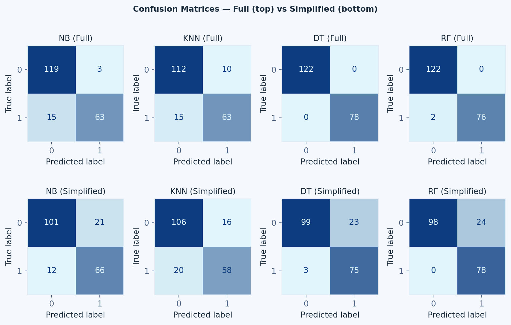
#| fig-cap: "Confusion matrices for all four models on the full (top) and simplified (bottom) datasets"
# --- Graphic 1: Confusion Matrices ---
fig, axes = plt.subplots(2, 4, figsize=(9, 5.85))
fig.suptitle('Confusion Matrices — Full (top) vs Simplified (bottom)',
fontsize=10, fontweight='bold', color=PALETTE['text'])
for idx, name in enumerate(models.keys()):
for row, (est, Xt, yt) in enumerate([
(trained_full[name], X_test, y_test),
(trained_simple[name], X_test_s, y_test_s),
]):
disp = ConfusionMatrixDisplay.from_estimator(
est, Xt, yt,
ax=axes[row, idx],
colorbar=False,
cmap=mpl.colors.LinearSegmentedColormap.from_list(
'bp', [PALETTE['accent_subtle'], PALETTE['primary_dark']]
)
)
axes[row, idx].set_title(
f'{name} ({"Full" if row == 0 else "Simplified"})',
fontsize=10, color=PALETTE['text']
)
plt.tight_layout()
plt.show()
```
#### ML Model Performance per Dataset Comparison
```{python}
#| eval: true
#| echo: false
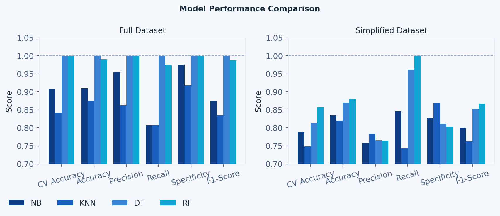
# --- Graphic 2: Metrics Comparison (per dataset) ---
metrics = ['CV Accuracy', 'Accuracy', 'Precision', 'Recall', 'Specificity', 'F1-Score']
model_names = list(models.keys())
x, width = np.arange(len(metrics)), 0.2
fig, axes = plt.subplots(1, 2, figsize=(9, 3.5))
fig.suptitle('Model Performance Comparison',
fontsize=10, fontweight='bold', color=PALETTE['text'])
bars = []
for i, name in enumerate(model_names):
b0 = axes[0].bar(x + i * width,
[results_full_df.loc[name, m] for m in metrics],
width, color=MODEL_COLORS[i], label=name)
axes[1].bar(x + i * width,
[results_simple_df.loc[name, m] for m in metrics],
width, color=MODEL_COLORS[i])
bars.append(b0[0])
for ax, title in zip(axes, ['Full Dataset', 'Simplified Dataset']):
ax.set_title(title, fontsize=10, color=PALETTE['text'])
ax.set_xticks(x + width * 1.5)
ax.set_xticklabels(metrics, rotation=15)
ax.set_ylim(0.7, 1.05)
ax.set_ylabel('Score')
ax.axhline(y=1.0, color=PALETTE['muted'], linestyle='--', linewidth=0.8)
# Single legend bottom-left of figure
fig.legend(bars, model_names,
loc='lower left', bbox_to_anchor=(0.01, -0.08),
ncol=4, frameon=False, fontsize=10)
plt.tight_layout()
plt.show()
```
#### Dataset Performance per ML Model Comparison
```{python}
#| eval: true
#| echo: false
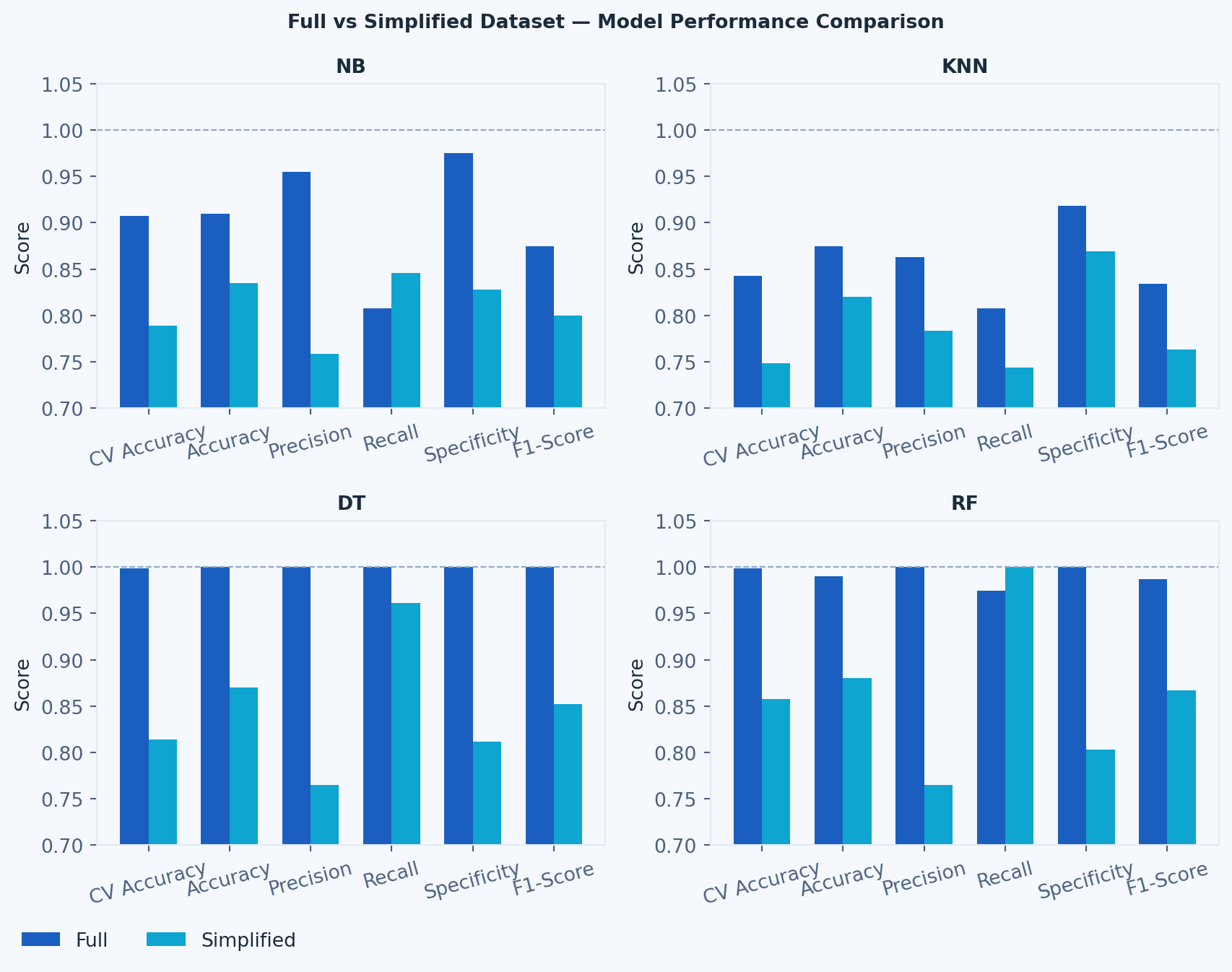
# --- Graphic 3: Full vs Simplified per Model ---
fig, axes = plt.subplots(2, 2, figsize=(9, 6.75))
fig.suptitle('Full vs Simplified Dataset — Model Performance Comparison',
fontsize=10, fontweight='bold', color=PALETTE['text'])
width = 0.35
bar_full = bar_simp = None
for idx, name in enumerate(model_names):
ax = axes[idx // 2, idx % 2]
bar_full = ax.bar(x - width/2,
[results_full_df.loc[name, m] for m in metrics],
width, color=PALETTE['primary'], label='Full')
bar_simp = ax.bar(x + width/2,
[results_simple_df.loc[name, m] for m in metrics],
width, color=PALETTE['accent'], label='Simplified')
ax.set_title(name, fontsize=10, fontweight='bold', color=PALETTE['text'])
ax.set_xticks(x)
ax.set_xticklabels(metrics, rotation=15)
ax.set_ylim(0.7, 1.05)
ax.set_ylabel('Score')
ax.axhline(y=1.0, color=PALETTE['muted'], linestyle='--', linewidth=0.8)
# Single legend bottom-left of figure
fig.legend([bar_full, bar_simp], ['Full', 'Simplified'],
loc='lower left', bbox_to_anchor=(0.01, -0.04),
ncol=2, frameon=False, fontsize=10)
plt.tight_layout()
plt.show()
```
#### Interactive Metrics Chart
```{python}
#| eval: true
#| echo: true
#| code-fold: true
#| code-summary: "Show — Interactive Metrics Chart"
#| fig-cap: "Interactive bar chart — hover to compare model metrics across full and simplified datasets"
metrics_list = ['CV Accuracy', 'Accuracy', 'Precision', 'Recall', 'Specificity', 'F1-Score']
model_names  = list(models.keys())

fig = make_subplots(rows=1, cols=2,
                    subplot_titles=['Full Dataset', 'Simplified Dataset'])

for i, name in enumerate(model_names):
    color = MODEL_COLORS[i]
    fig.add_trace(go.Bar(
        name=name,
        x=metrics_list,
        y=[results_full_df.loc[name, m] for m in metrics_list],
        marker_color=color,
        legendgroup=name,
        showlegend=True
    ), row=1, col=1)
    fig.add_trace(go.Bar(
        name=name,
        x=metrics_list,
        y=[results_simple_df.loc[name, m] for m in metrics_list],
        marker_color=color,
        legendgroup=name,
        showlegend=False
    ), row=1, col=2)

fig.update_layout(
    barmode='group',
    plot_bgcolor=PALETTE['surface'],
    paper_bgcolor=PALETTE['surface'],
    font=dict(color=PALETTE['text'], size=10),
    legend=dict(orientation='h', y=-0.2),
    margin=dict(l=0, r=0, t=30, b=0),
    yaxis=dict(range=[0.7, 1.05]),
    yaxis2=dict(range=[0.7, 1.05]),
)
fig.show()
```
### The Original Code
#### 1. Imports
*All libraries imported at the top of the file to avoid duplication and ensure a clear dependency overview.*
```python
# SECTION 1 — IMPORTS

import pandas as pd
import numpy as np
import matplotlib.pyplot as plt

from sklearn.preprocessing import LabelEncoder, OrdinalEncoder, StandardScaler
from sklearn.model_selection import train_test_split, cross_val_score, StratifiedKFold
from sklearn.metrics import (accuracy_score, precision_score, recall_score,
                             f1_score, confusion_matrix, ConfusionMatrixDisplay)
from sklearn.naive_bayes import GaussianNB
from sklearn.neighbors import KNeighborsClassifier
from sklearn.tree import DecisionTreeClassifier
from sklearn.ensemble import RandomForestClassifier
```
#### 2. Dataset and Data Preparation
*Loads the CSV, encodes binary/ordinal/categorical variables, performs 80–20 train-test split, standardises numerical features, and creates the simplified dataset by removing the five clinically restricted attributes.*
```python
# SECTION 2 — DATASET AND DATA PREPARATION

# --- Load Dataset ---
df = pd.read_csv('/Users/tom.bme/Projects/heart_disease_dataset.csv',
                 sep=';',
                 keep_default_na=False)

print(df.shape)
print(df.isnull().sum())
print(df.dtypes)

# --- Define Features & Target ---
X = df.drop(columns=['Heart Disease'])
y = df['Heart Disease']

# --- Encode Binary Variables (0/1) ---
binary_cols = ['Gender', 'Family History', 'Diabetes', 'Obesity', 'Exercise Induced Angina']
le = LabelEncoder()
for col in binary_cols:
    X[col] = le.fit_transform(X[col])

# --- Encode Ordinal Variables (preserve order) ---
oe_smoking = OrdinalEncoder(categories=[['Never', 'Former', 'Current']])
X[['Smoking']] = oe_smoking.fit_transform(X[['Smoking']])

oe_alcohol = OrdinalEncoder(categories=[['None', 'Moderate', 'Heavy']])
X[['Alcohol Intake']] = oe_alcohol.fit_transform(X[['Alcohol Intake']])

# Stress Level is already numeric (1–10) — no encoding needed

# --- Encode Categorical Variables (one-hot) ---
X = pd.get_dummies(X, columns=['Chest Pain Type'])

# --- Clean up dtypes ---
chest_pain_cols = ['Chest Pain Type_Asymptomatic', 'Chest Pain Type_Atypical Angina',
                   'Chest Pain Type_Non-anginal Pain', 'Chest Pain Type_Typical Angina']
X[chest_pain_cols]    = X[chest_pain_cols].astype(int)
X['Smoking']          = X['Smoking'].astype(int)
X['Alcohol Intake']   = X['Alcohol Intake'].astype(int)

# --- Full Dataset: Train-Test Split & Standardisation ---
X_train, X_test, y_train, y_test = train_test_split(
    X, y, test_size=0.2, random_state=42, stratify=y
)

numerical_cols = ['Age', 'Cholesterol', 'Blood Pressure', 'Heart Rate',
                  'Exercise Hours', 'Blood Sugar']

scaler = StandardScaler()
X_train[numerical_cols] = scaler.fit_transform(X_train[numerical_cols])
X_test[numerical_cols]  = scaler.transform(X_test[numerical_cols])

# --- Simplified Dataset: Remove features requiring professional equipment ---
cols_to_drop = ['Cholesterol', 'Blood Sugar', 'Diabetes',
                'Exercise Induced Angina',
                'Chest Pain Type_Asymptomatic',
                'Chest Pain Type_Atypical Angina',
                'Chest Pain Type_Non-anginal Pain',
                'Chest Pain Type_Typical Angina']

X_simple = X.drop(columns=cols_to_drop)
numerical_simple = ['Age', 'Blood Pressure', 'Heart Rate', 'Exercise Hours']

X_train_s, X_test_s, y_train_s, y_test_s = train_test_split(
    X_simple, y, test_size=0.2, random_state=42, stratify=y
)

scaler_s = StandardScaler()
X_train_s[numerical_simple] = scaler_s.fit_transform(X_train_s[numerical_simple])
X_test_s[numerical_simple]  = scaler_s.transform(X_test_s[numerical_simple])
```
#### 3. Classification Algorithms and Evaluation
*Defines NB, KNN, DT, and RF with their tuning parameters. Applies 5-fold stratified CV and computes all six evaluation metrics for both the full and simplified datasets.*
```python
# SECTION 3 — CLASSIFICATION ALGORITHMS & EVALUATION

# --- Define Models ---
models = {
    'NB':  GaussianNB(),
    'KNN': KNeighborsClassifier(n_neighbors=5, metric='euclidean'),
    'DT':  DecisionTreeClassifier(max_depth=5, min_samples_split=10, random_state=42),
    'RF':  RandomForestClassifier(n_estimators=100, max_depth=5, random_state=42),
}

cv = StratifiedKFold(n_splits=5, shuffle=True, random_state=42)

# --- Evaluation Function ---
def evaluate(models, X_tr, X_te, y_tr, y_te, cv):
    results = {}
    for name, model in models.items():
        cv_scores = cross_val_score(model, X_tr, y_tr, cv=cv, scoring='accuracy')
        model.fit(X_tr, y_tr)
        y_pred = model.predict(X_te)
        tn, fp, fn, tp = confusion_matrix(y_te, y_pred).ravel()
        results[name] = {
            'CV Accuracy': round(cv_scores.mean(), 4),
            'CV Accuracy SD': round(cv_scores.std(), 4),
            'Accuracy':    round(accuracy_score(y_te, y_pred), 4),
            'Precision':   round(precision_score(y_te, y_pred), 4),
            'Recall':      round(recall_score(y_te, y_pred), 4),
            'Specificity': round(tn / (tn + fp), 4),
            'F1-Score':    round(f1_score(y_te, y_pred), 4),
        }
    return pd.DataFrame(results).T

# --- Run Evaluation ---
results_full_df   = evaluate(models, X_train,   X_test,   y_train,   y_test,   cv)
results_simple_df = evaluate(
    {name: type(m)(**m.get_params()) for name, m in models.items()},
    X_train_s, X_test_s, y_train_s, y_test_s, cv
)

print("=== FULL DATASET ===")
print(results_full_df)
print("\n=== SIMPLIFIED DATASET ===")
print(results_simple_df)
```
#### 4. Evaluation Graphics
*Generates three figures: confusion matrices (full vs simplified), grouped metrics bar charts per dataset, and side-by-side full vs simplified comparison per model.*
```python
# SECTION 4 — EVALUATION GRAPHICS

# --- Retrain models for plotting ---
trained_full, trained_simple = {}, {}
for name, model in models.items():
    model.fit(X_train, y_train)
    trained_full[name] = model
    model_s = type(model)(**model.get_params())
    model_s.fit(X_train_s, y_train_s)
    trained_simple[name] = model_s

# --- Graphic 1: Confusion Matrices ---
fig, axes = plt.subplots(2, 4, figsize=(20, 9))
fig.suptitle('Confusion Matrices — Full (top) vs Simplified (bottom)', fontsize=14, fontweight='bold')
for idx, name in enumerate(models.keys()):
    ConfusionMatrixDisplay.from_estimator(trained_full[name],   X_test,   y_test,   ax=axes[0, idx])
    ConfusionMatrixDisplay.from_estimator(trained_simple[name], X_test_s, y_test_s, ax=axes[1, idx])
    axes[0, idx].set_title(f'{name} (Full)')
    axes[1, idx].set_title(f'{name} (Simplified)')
plt.tight_layout()
plt.savefig('confusion_matrices.png', dpi=150)
plt.show()

# --- Graphic 2: Metrics Comparison (per dataset) ---
metrics      = ['CV Accuracy', 'Accuracy', 'Precision', 'Recall', 'Specificity', 'F1-Score']
model_names  = list(models.keys())
x, width     = np.arange(len(metrics)), 0.2

fig, axes = plt.subplots(1, 2, figsize=(18, 6))
fig.suptitle('Model Performance Comparison', fontsize=14, fontweight='bold')
for i, name in enumerate(model_names):
    axes[0].bar(x + i * width, [results_full_df.loc[name, m]   for m in metrics], width, label=name)
    axes[1].bar(x + i * width, [results_simple_df.loc[name, m] for m in metrics], width, label=name)
for ax, title in zip(axes, ['Full Dataset', 'Simplified Dataset']):
    ax.set_title(title)
    ax.set_xticks(x + width * 1.5)
    ax.set_xticklabels(metrics, rotation=15)
    ax.set_ylim(0.7, 1.05)
    ax.set_ylabel('Score')
    ax.legend()
    ax.axhline(y=1.0, color='grey', linestyle='--', linewidth=0.8)
plt.tight_layout()
plt.savefig('metrics_comparison.png', dpi=150)
plt.show()

# --- Graphic 3: Full vs Simplified per Model ---
fig, axes = plt.subplots(2, 2, figsize=(16, 12))
fig.suptitle('Full vs Simplified Dataset — Model Performance Comparison', fontsize=14, fontweight='bold')
width = 0.35
for idx, name in enumerate(model_names):
    ax = axes[idx // 2, idx % 2]
    ax.bar(x - width/2, [results_full_df.loc[name, m]   for m in metrics], width, label='Full',       color='steelblue')
    ax.bar(x + width/2, [results_simple_df.loc[name, m] for m in metrics], width, label='Simplified', color='coral')
    ax.set_title(name, fontsize=13, fontweight='bold')
    ax.set_xticks(x)
    ax.set_xticklabels(metrics, rotation=15)
    ax.set_ylim(0.7, 1.05)
    ax.set_ylabel('Score')
    ax.legend()
    ax.axhline(y=1.0, color='grey', linestyle='--', linewidth=0.8)
plt.tight_layout()
plt.savefig('full_vs_simplified.png', dpi=150)
plt.show()
```